Let’s delve into a real-world project to grasp the practical implications of these techniques. Our challenge was predicting the duration between ticket updates (‘sys_update_at’) and their closing time (‘closed_at’) in an IT service setting. Each unique incident ticket was denoted by an identifier ‘number’. Each row with the same number represents a certain update to that ticket. There are columns that represent information that are only uncovered through investigation sometime in the middle of the ticket’s lifespan. However, in our dataset, this information is propagated to all rows of that incident ticket. Given that we do not have the specifics about which stage were these columns should’ve been first available, we will be excluding these columns.
Exploratory Data Analysis
The following are the findings of our brief exploratory data analysis:
“New” and “Active” ticket states have more than 30,000 rows each. Note that this counts update instances with that state, and not just unique ticket numbers. Tickets can cycle between states throughout its life cycle.

While very few, tickets that are Awaiting Evidence and Awaiting Vendor has a very huge range of values to the days before they were finally closed. This is expected as these states are usually out of the hands of the service team. It is noteworthy that once a ticket is “Resolved” it will be closed in about 5 days. The variation is too small to be visible. This implies some rule-based closing.

Ticket numbers with outlier durations were removed. See below that “Awaiting Vendor” state has been less varied, and “Awaiting Evidence” state has been completely removed.

When splitting using Ticket priority, it can be seen that higher priority tickets get closed faster, but not by much. This might imply that higher priority tickets are also more complex so everything roughly evens out the a median of about 9 days.

We will also be excluding tickets that never reached the ‘Resolved’ state. For the final dataset, the ‘Closed’ states of the tickets were also removed as there is no longer a need to predict at that stage. Our final dataset contains about 19,200 unique incident tickets, down from the original 20,700.
Building the Predictive Model
Constructing a predictive model involves a series of systematic steps, and Scikit-Learn pipelines simplify this process.
- Datetime Feature Extraction: Dissected date and time variables for nuanced temporal insights.
- Target Encoding: Enhanced the model’s understanding of categorical data.
- Handling Missing Data: Imputed missing values intelligently using the ‘most_frequent’ strategy.
- Feature Selection: Variance Threshold ensured the model focused on significant features, enhancing prediction accuracy.
- Model Selection: XGBoost Regressor, a robust gradient boosting algorithm, was employed for its adaptability and efficiency.

Transformer Implementation
The code below shows how the feature engineering steps were implemented in Scikit-learn. For the target encoding, we encode categories by the mean of the target variable for that category. See that we only compute the mean during the “fit” step. That value is saved, and when we “transform” the test data, we just use the pre-calculated values from the training set.
Evaluating Model Performance
To split the data between training and testing, we sorted it via creation date and ticket number. The older tickets will be used to predict newer tickets. No rows with the same ‘number’ will be split between the two. A baseline “naive” model is constructed by randomly picking values from a Poisson distribution with the same mean as the training data’s target column. This tries to mimic the distribution of values from the training set. We then measure its performance against the actual values by measuring the Root Mean Square Error and Mean Absolute Error.
Baseline Model:
RMSE: 5.33 days
MAE: 4.31 days
For the pipeline, we used random search to try out various combinations of hyperparameters that will yield the best results. You can see that we implemented a Group K-Fold. While the actual ‘number’ columns are not used by the XGBoost Regressor it is used to ensure that rows from the same ticket ‘number’ are not separated during cross validation.
Fine-Tuned Model:
RMSE: 3.63 days
MAE: 2.38 days
Using the trained pipeline cuts the average error by about half. If we compute the MAE per state, it goes even lower.


Build an Automated ETL Pipeline. From setting up Docker to utilizing APIs and automating workflows with GitHub Actions, this post goes through it all.

Ready to dive into data science? Learn how to set up your development environment using Docker for a seamless and reproducible workspace. Say goodbye to compatibility issues and hello to data science success!

In this short project, I scraped all of Lebron's regular season points and plotted them in an interactive graph.

In this project I analyzed a fitness center's attendance data to predict attendance rates of its group classes.

A marketing agency presents a promotional plan to a telecommunication company to increase its subscriber base and generate revenue. Using population and location data, we estimated the feasibility of this plan in this case study.

The tweet that started the trend was posted on June 12 (Philippine Independence day). On that tweet, the author stated that he dined in at a Tropical Hut branch, and he is their only customer. Despite the pandemic “restrictions”, commercial activity on malls and fast food chains are pretty much back to “normal”, so having only one customer is disheartening.

In this project I trained a transformer model to recognize words from audio.

In this article, I fine-tuned a pre-trained object detection model using a small custom dataset.

In this article, we will build a simple deep learning based demo application that can be accessed publicly in Hugging Face spaces

The rate at which unreliable news was spread online in the recent years was unprecedented. In this project, I finetuned some language models to make an unreliable news classifier.

In this article, we will discuss how to quickly showcase your model publicly as a machine learning application for free.

In this article, I will discuss a way of accessing Google Cloud GPUs to train your Deep Learning projects.

Code This case study is my capstone project for the Google Data Analytics Certification offered through Coursera. I was given access to …
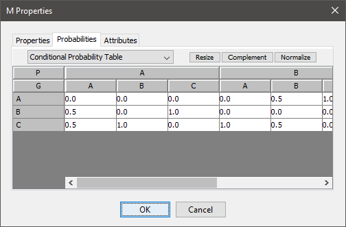
However, to make it a little bit more scalable, the tables are defined in a separate Google sheet, and imported into the Google Colab notebook. Each node is a separate worksheet, and the columns list the parent nodes, the name of the node, and probability.
Bayesian Networks are a compact graphical representation of how random variables depend on each other. It can be used to demonstrate the …

In this article we will break down what the Fourier Transform does to a signal, then we will be using Python to compute and visualize the transforms of different waveforms.