Keyword Spotting is recognizing an uttered word from an audio clip. It’s input data is a waveform, and its output is the classification. In this project, I converted 1-d audio waveform to a 2-d mel-spectrogram. The horizontal axis of a spectrogram is time (in frames) and the vertical axis is frequency. The mel-spectrogram gives more “detail” to some frequencies to closer match human hearing. I have a more detailed discussion regarding spectrograms here.
Now that the input data is 2-dimensional, the project is now very similar to an image classification problem. Convolutional neural networks, which are very successful in the vision domain can be applied to audio/speech using this spectrogram conversion. In this project however, I tried to use transformers which were popular in the natural language domain, and have since been adapted in the vision domain.
When using transformers for images, the input image is typically split into a series of smaller image patches by using a 2-dimensional grid. For example a 256×256 pixel image, split using a 16×16 grid will result into patches of 16×16 pixels.

I initially patchified my images this way and got 83% accuracy on the test set. The difference of a spectrogram with a natural image is that it already has an inherent sequential property. As stated earlier, the horizontal axis conveys time. After reading this paper by Berg et. al, I changed the patch grid size to be 1-dimensional. My patches are now of the size 128×2 “pixels”. This means I preserved the frequency axis and each patch contains two frames of the spectrogram.
I played around with different training hyperparameters and adding dropout layers to finally reach a test accuracy of 93.5%. The short video below is a sample demonstration application to showcase the model.
Other Articles
In this article, I fine-tuned a pre-trained object detection model using a small custom dataset.
In this article, we will discuss how to quickly showcase your model publicly as a machine learning application for free.
Unlocking Data Science: Your Easy Docker Setup Guide
Ready to dive into data science? Learn how to set up your development environment using Docker for a seamless and reproducible workspace. Say goodbye to compatibility issues and hello to data science success!
In this article, I will discuss a way of accessing Google Cloud GPUs to train your Deep Learning projects.
Mastering Pipelines: Integrating Feature Engineering into Your Predictive Models
Master predictive modeling with Scikit-Learn pipelines. Learn the importance of feature engineering and how to prevent data leakage.
Build an Automated ETL Pipeline. From setting up Docker to utilizing APIs and automating workflows with GitHub Actions, this post goes through it all.
However, to make it a little bit more scalable, the tables are defined in a separate Google sheet, and imported into the Google Colab notebook. Each node is a separate worksheet, and the columns list the parent nodes, the name of the node, and probability.
Predicting a Fitness Center’s Class Attendance with Machine Learning
In this project I analyzed a fitness center's attendance data to predict attendance rates of its group classes.
In this short project, I scraped all of Lebron's regular season points and plotted them in an interactive graph.
A marketing agency presents a promotional plan to a telecommunication company to increase its subscriber base and generate revenue. Using population and location data, we estimated the feasibility of this plan in this case study.
In this article we will break down what the Fourier Transform does to a signal, then we will be using Python to compute and visualize the transforms of different waveforms.
Fast and Free Deep Learning Demo with Gradio
In this article, we will build a simple deep learning based demo application that can be accessed publicly in Hugging Face spaces
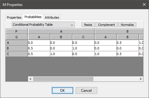