
I have created an attendance rate column by dividing the attendance number with the class capacity. I then computed the correlation of the numerical features with attendance rate.

I also used qq-plots to see if the columns are normally distributed.

For the categorical columns, I have used a boxplot to show the distribution of attendance rates across each category.

The following were some of my insights:
- 75% of the class have less than 66% attendance rate (75th percentile)
- Using the histogram of the pairplot, attendance rates are almost uniformly distributed with a few outlier values. Age, new members, and over 6 month members, follow a normal distribution. The qq-plot also confirm this close to normal distribution as they fit the normal-line closely.
- From both the scatterplot in the pairplot, and the correlation computation, classes with higher average ages tend to have low attendance rates (negative correlation), and classes with higher sign-ups (both new and over 6 month members) tend to have higher attendance rates (positive correlation).
- The distribution of attendance rates has been broken down across categories using box plots.
- Tuesdays and Fridays have higher median attendance rates
- Attendance rates between AM and PM classes are very similar.
- In terms of class activity, strength and yoga classes have higher attendance rates while cycling have the lowest.
Evaluation Strategy
- First, I have set aside 10% of my data as a final test set. I then create a naive model that constantly outputs the mean attendance rate of the training data.
- Next, for validation, I used 10-Fold validation (repeated 3 times). Since the data set is small and the models that are chosen aren’t very computationally expensive, I validated the models on random subsets multiple times to generate a distribution of model performance. This has shown me not only the average error but also spread. I am looking for a model that has low average error and small spread.
- Finally, I fit the models on the whole dataset and then tested them against the held out test set to see its performance on never before seen data.
Metric
- I have chosen to use root mean square error as my evaluation metric.
- It is a very popular metric used for regression problems. It measure the distance of the predictions from the correct values and it penalizes very far-off predictions.

Outcome
- All models performed better than the naive model.
- For both the validation and testing, the fine tuned Ridge Regression model comes out on top, but it is only better by about 0.001.
- The Random Forest model was not able to outperform the linear models.
- Since we predicted attendance rates, if we transform it back to number of students, our model’s prediction can be off by 2-3 students.
- I choose the Ridge Regression model as the better performing approach. At the scale of the dataset it is not much more complex as compared to linear regression, and by fine-tuning we can get slightly better performance.


Master predictive modeling with Scikit-Learn pipelines. Learn the importance of feature engineering and how to prevent data leakage.

In this project I trained a transformer model to recognize words from audio.

The tweet that started the trend was posted on June 12 (Philippine Independence day). On that tweet, the author stated that he dined in at a Tropical Hut branch, and he is their only customer. Despite the pandemic “restrictions”, commercial activity on malls and fast food chains are pretty much back to “normal”, so having only one customer is disheartening.

In this short project, I scraped all of Lebron's regular season points and plotted them in an interactive graph.

In this article we will break down what the Fourier Transform does to a signal, then we will be using Python to compute and visualize the transforms of different waveforms.

Code This case study is my capstone project for the Google Data Analytics Certification offered through Coursera. I was given access to …

In this article, we will discuss how to quickly showcase your model publicly as a machine learning application for free.

Build an Automated ETL Pipeline. From setting up Docker to utilizing APIs and automating workflows with GitHub Actions, this post goes through it all.

Ready to dive into data science? Learn how to set up your development environment using Docker for a seamless and reproducible workspace. Say goodbye to compatibility issues and hello to data science success!

The rate at which unreliable news was spread online in the recent years was unprecedented. In this project, I finetuned some language models to make an unreliable news classifier.

In this article, I will discuss a way of accessing Google Cloud GPUs to train your Deep Learning projects.
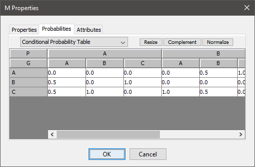
However, to make it a little bit more scalable, the tables are defined in a separate Google sheet, and imported into the Google Colab notebook. Each node is a separate worksheet, and the columns list the parent nodes, the name of the node, and probability.

In this article, we will build a simple deep learning based demo application that can be accessed publicly in Hugging Face spaces

A marketing agency presents a promotional plan to a telecommunication company to increase its subscriber base and generate revenue. Using population and location data, we estimated the feasibility of this plan in this case study.
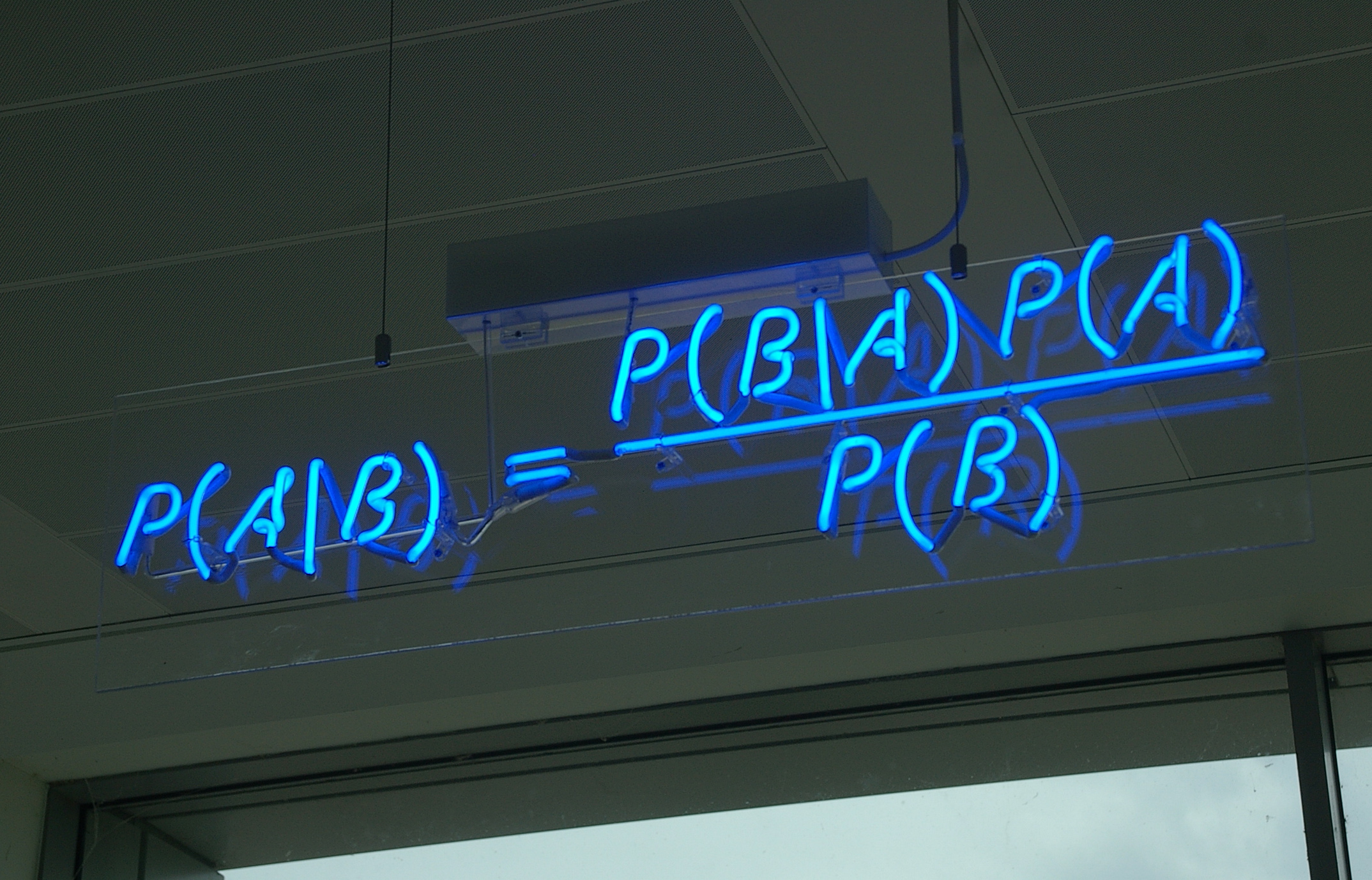
Bayesian Networks are a compact graphical representation of how random variables depend on each other. It can be used to demonstrate the …
In this article, I fine-tuned a pre-trained object detection model using a small custom dataset.